Contrast Enhancement through Localized Histogram Equalization
Histogram Equalization for Image Enhancement
Here is the problem stated very simply — some pictures have poor distributions of brightness values.
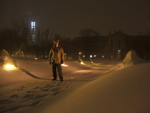
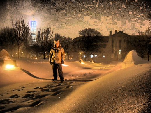
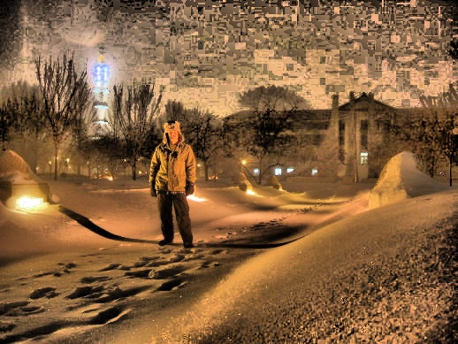
See the example below, a picture of myself on the Purdue University campus after a snow storm. The original image from my digital camera was 2592x1944, this is the result of downsampling that original by a factor of 5 to 518x389.
A simple complaint about this image might be that too much of it is the same thing or very nearly the same thing. That is, large expanses of browns and ambers. There is a large light amber snowbank in the right foreground, a dark brown and largely featureless building in the distance at right, and the top quarter to third of the image is a light brown sky.
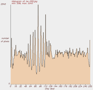
That same complaint in mathematical form might be that the histogram of its brightness values is very non-uniform. See that histogram below. The horizontal axis is the range of possible brightness values. The vertical axis indicates the number of pixels taking each of those possible brightness values.
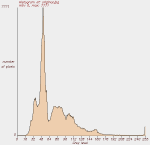
Possible brightness values range from 0 through 255. Almost all of the points in the image are at brightnesses below 128, half the possible brightness. A small number of pixels are in the range of 250 through 255, those being the lights along the walkway where I'm standing, the lights in the main door and the ground floor windows of the building, and on the distant bell tower. From brightness values 176 through 250 there are almost no points in the image with those brightnesses.
Meanwhile the majority of the image is lumped together at very similar brightnesses. Put another way, most points in the image look very much like most of the rest of the points in the image.
Histogram equalization is a technique for recovering some of apparently lost contrast in an image by remapping the brightness values in such a way as to equalize, or more evenly distribute, its brightness values. As a side effect, the histogram of its brightness values becomes flatter.
A C/C++ program for histogram equalization can easily written using the Open Computer Vision Library or OpenCV. The major steps of such a program include:
1 —
Read the input image.
This can be in most any image format thanks to
OpenCV.
This input image contains n pixels:
n = height × width
2 — Convert from RGB (curiously stored in the order blue, green, red by OpenCV) to HSV: Hue, Saturation, and Value. Value is what I've been informally calling "brightness" here. See, for example, the useful discussion on the Wikipedia page for the difference between HSV and HSI, and the differences between the meanings for the terms lightness, luminance, luminosity, intensity, and value, as well as clear explanations of conversions between the R,G,B and H,S,V color spaces.
3 — Calculate the histogram of the input image. This is a 256 value array, where H[x] contains the number of pixels with value x.
4 —
Calculate the cumulative density function
of the histogram.
This is a 256 value array, where cdf[x] contains
the number of pixels with value x or less:
cdf[x] = H[0] + H[1] + H[2] + ... + H[x]
5 —
Loop through the n pixels in the entire image and
replace the value at each i'th point:
V[i] <-- floor(255*(cdf[V[i]] - cdf[0])/(n - cdf[0]))
6 — Convert the image back from HSV to RGB.
7 — Save the image in the desired format and file name.
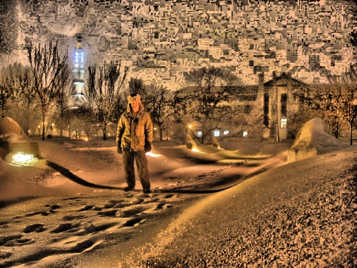
Below is the result of histogram equalization of the original image. Notice the improvements:
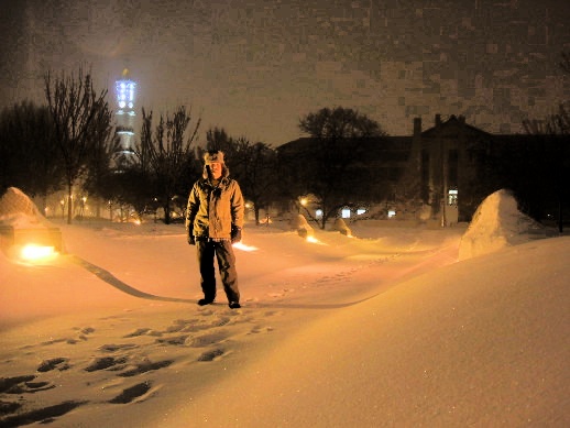

Here is a half-sized copy of the original for comparison. Notice:
1: The snow has become lighter, revealing some details of the footprints.
2: The building at right has become darker, increasing its contrast against the lighter snow and sky. The four-story fountain in front of the center of that building is become a bit more visible.
3: Details on the bell tower have become more distinct.
4: The distant lighted area beneath and beyond the trees at left, below and to the left of the bell tower, has become more distinct.
There are, of course, trade-offs. Notice how the contrast stretching in the sky has brought out some blocky artifacts caused by the camera's JPEG encoding of the original image. Those artifacts are in the original, but they are not visible in that rather murky image.
The first image here is the histogram of the original image again, the second is the histogram of the enhanced image.
Histogram of original image, again.
Histogram of enhanced image — not flat, but flatter.
The resulting histogram is not flat, but it is much more evenly distributed than the original.
Remember that any two pixels with identical values in the original must have identical values in the output. At some adequately fine scale, collections of one or a few adjacent histogram bins in the output will not have the same pixel counts.
Dithering could be used. That is the addition or subtraction of a small pseudorandom value to the output pixel's value to force a flatter final histogram. However, dithering obviously adds random noise to the image. It degrades scientific data and seems to add no real esthetic improvement to the resulting appearance. A small dither in the range of -1.0 through +1.0 applied before the remapping might somewhat obscure the blocky JPEG artifacts in the sky, but that would be the only difference.
Below is a simple result for more scientific data, registered intensity data from a structured-light 3-D scan of a narrow band on a cuneiform tablet:
Input image (a portion of a cuneiform tablet).
Result of histogram equalization.
To enhance the contrast of a color image, you could simply apply histogram equalization to the red, green, and blue color planes.
Alternatively, convert the R,G,B data to H,S,I (Hue, Saturation, Intensity), apply histogram equalization to the intensity channel only, and convert back to R,G,B.
The Remaining Problem
Images typically have both large-scale and small-scale variation in intensity, representing features of varying sizes. From an image-processing perspective, an image contains information at varying frequencies, bounded at the low and high ends by the overall image dimensions and the pixel spacing, respectively. Conventional histogram equalization can improve the visibility of local (high-frequency) features only within limits imposed by the overall (low-frequency) variation.
The above image pairs demonstrate this — the input images have large-scale variations at periods one to two times the size of the image. The snow scene is lightest across its bottom third, darkest across its middle third, and slightly lighter again across its top this. The cuneiform image varies from dimmest at upper-left to brightest at lower-right. The local contrast is improved throughout the images, but not as much as could be possible.
If the image could be segmented into self-similar regions, a histogram could be constructed for each region, and applied for remapping only the pixels within its region. But the image above indicates that large-scale variation will frequently be relatively smooth and not amenable to segmentation.
One Possible Solution — Localized Histogram Equalization
As a simple solution, we can apply histogram equalization independently to small regions of the image. Most small regions will be very self-similar. If the image is made up of discrete regions, most small regions will lie entirely within one or the other region. If the image has more gradual large-scale variation, most small regions will contain only a small portion of the large-scale variation.
JPEG compression discards some information. Localized histogram equalization on the snow scene leads distracting levels of JPEG artifacts, as you will see further down.
Let's start with non-lossy input!
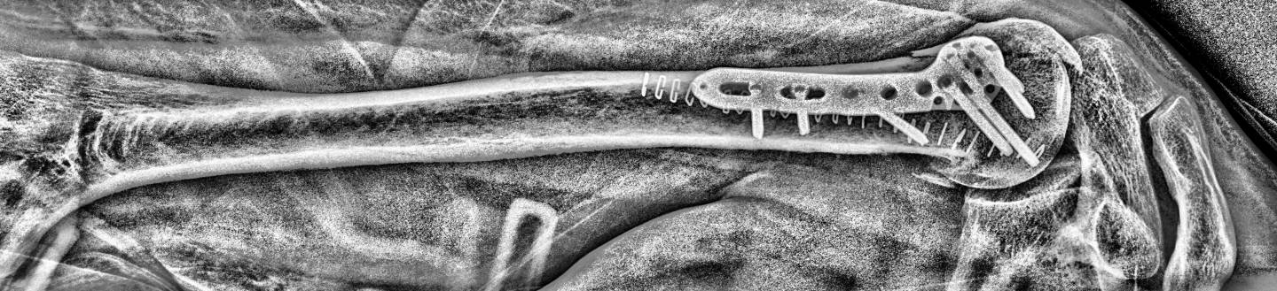
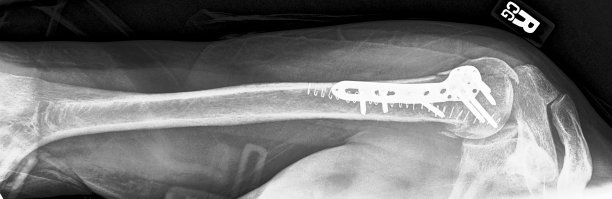
The first image here is an X-ray image of an upper right arm, elbow at left and shoulder at right, downsampled to 15% of its original size of 4078x1328 pixels.
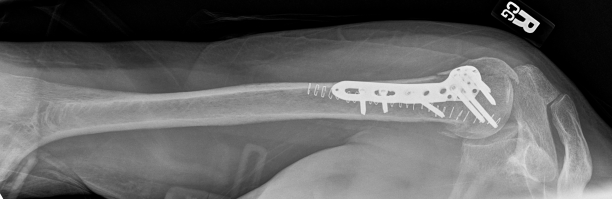
Original X-ray image downsampled to just 15% of original size.
Original xray with global histrogram equalization applied, then downsampled to 15% of original size.
I have written software to remap each pixel based on the histogram of the circular region centered at that pixel. Now let's see the result of histogram equalization performed uniquely for each pixel based on its circular neighborhood with radii of 320, 160, 80, 40, 20 and 10 pixels, and the resulting image downsampled by 50%. The wire staples are about 7 to 8 pixels wide in the original image.
First, toward the distal (elbow) end showing the internal structure of the bone:
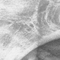
Sample from distal end after global equalization of image.
Sample from distal end after localized histogram equalization over a 320-pixel radius centered at each pixel.
Sample from distal end after localized histogram equalization over a 160-pixel radius centered at each pixel.
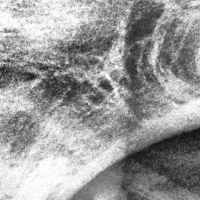
Sample from distal end after localized histogram equalization over a 80-pixel radius centered at each pixel.
Sample from distal end after localized histogram equalization over a 40-pixel radius centered at each pixel.
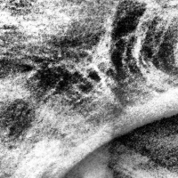
Sample from distal end after localized histogram equalization over a 20-pixel radius centered at each pixel.
Sample from distal end after localized histogram equalization over a 10-pixel radius centered at each pixel.
And now the proximal (shoulder) end, with the repair hardware:
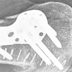
Sample from proximal end after global equalization of image.
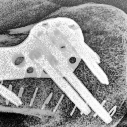
Sample from proximal end after localized histogram equalization over a 320-pixel radius centered at each pixel.
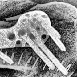
Sample from proximal end after localized histogram equalization over a 160-pixel radius centered at each pixel.
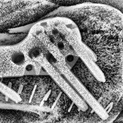
Sample from proximal end after localized histogram equalization over a 80-pixel radius centered at each pixel.
Sample from proximal end after localized histogram equalization over a 40-pixel radius centered at each pixel.
Sample from proximal end after localized histogram equalization over a 20-pixel radius centered at each pixel.
Sample from proximal end after localized histogram equalization over a 10-pixel radius centered at each pixel.
Now similar processing of the snow scene, with radii of 100, 50, and 25 pixels. The input is a JPEG image, so we will see blocky quantization.
Original image, again.
Global histogram equalization, again.
Localized histogram equalization, radius of 100 pixels. Notice how the footprints and the graininess of the nearest snow bank are accentuated. The roughly triangular fountain components are more district from the building than they are in the global enhancement directly above. The horizontal bands of light masonry and the darker windows on that building have also become more distinct.
Localized histogram equalization, radius of 50 pixels. Further accentuation of the nearby snow texture, and the tree limbs become more distinct from their background. Building details become even sharper.
Localized histogram equalization, radius of 25 pixels. The high-pass filter effect becomes even more noticeable, and the building seems more visible through the thinning trees.
The JPEG artifacts in the sky become more pronounced as the equalization radius decreases. So, lesson learned, capture low-light images in "raw" mode and do not let the camera introduce distracting artifacts caused by lossy JPEG compression.
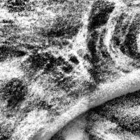
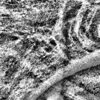
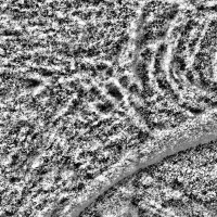
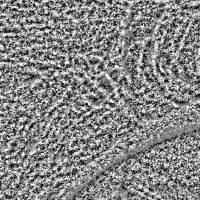
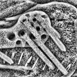
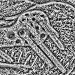
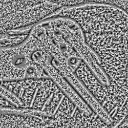
Below is similar processing applied to the cuneiform image. Again it's the original input image, global histogram equalization, then localized histogram equalization at radii of 100, 50, 25, and 12 pixels:
Input image (a portion of a cuneiform tablet).
Global histogram equalization (i.e., all pixels are remapped with one histogram based on the entire image).
Histogram equalization based on a region of radius of 100 pixels.
Histogram equalization based on a region of radius of 50 pixels.
Histogram equalization based on a region of radius of 25 pixels.
Histogram equalization based on a region of radius of 12 pixels:
The last image is not particularly useful, but the other results of localized histogram equalization show what I think are improved visualization. Compared to the global histogram equalization, radii of 100, 50, and 25:
- Improve the contrast between the signs at the right and their background.
- Sharpen the signs at right.
- Increase the contrast in the unused portion of the tablet at left.
Localized histogram equalization is obviously a form of high-pass filtering, in which low-frequency information (large-scale intensity variation) is blocked.
Now for the bad news.... The computational complexity increases with order O(n2m2) with image length and width of n pixels and region radius of m pixels. The radii used in these examples were chosen to double in size, and so each step quadrupled in processing time. The 100-pixel radius enhancement takes approximately 64 times as long as the 12-pixel radius. Obviously field data collection would have to be separated from archival processing!
Data Used
The cuneiform tablet is item "Spalding 1, Ur III", on loan from Gordon Young. The input data was obtained by simply scanning the tablet on a flatbed document scanner at 600 dpi. Thumbnails of the original unenhanced scans are:
| Obverse face | Reverse face |
| 1st row | 1st row (over top edge) |
|
|
| 2nd row | 2nd row |
|
|
| 3rd row | 3nd row |
|
|
| 4th row | 4th and 5th row |
|
|
| 5th row | |
|
| Obverse 30 degrees | Reverse 45 degrees | Edge |
|
|
|
The 600 dpi resolution results in the following dimensions of the regions considered when remapping each pixel:
| Radius | Area | ||||
| pixels | inches | mm | pixels2 | inches2 | mm2 |
| 100 | 0.1667 | 4.2333 | 31415 | 0.08727 | 56.3008 |
| 50 | 0.08333 | 2.1167 | 7853 | 0.02182 | 14.0752 |
| 25 | 0.04167 | 1.0583 | 1963 | 0.005454 | 3.5188 |
| 12 | 0.02 | 0.508 | 452 | 0.001257 | 0.8107 |
Applications to radiological data
Applications to 3-D data visualization
References
The following provided the motivation and initial guidance: "Contrast Limited Adaptive Histogram Equalization," Karel Zuiderveld, Graphics Gems IV, Paul Heckbert, editor, Academic Press, 1994. However, that work described subdividing the image into 16x16 blocks, calculating the histogram of each such block, and interpolating between remappings for points.