Archival Data Format for 3-D Data Collection, Analysis, and Applications
Archival Data Format
The data storage format has been a matter of some concern. We require maximum portability, long-term utility, efficient searching of an archive for data of interest, and efficient storage. For maximum portability and long-term utility, we store our initial sensor data as ASCII data. The ASCII format, and the header described below, provide for efficient searching of archives. Run-length encoding is used for efficient storage. Each archival file starts with a human-readable header describing meta-information:
Sensor data characteristics including the number of rows and columns in the range map, and a calibration matrix to convert the stored sensor data to (x,y,z) vectors. Note that this matrix determines theoretical limits on resolution.
Measurement session characteristics including the time and date of data collection, user and system gathering the data, user-provided specimen description, and sensor configuration.
Explanations of how to decode the sensor data, convert it to (x,y,z) vectors with registered intensity values, and assemble them into a range map. This includes:
- How to decode the run-length encoding.
- How each data point encodes both position and registered intensity. By "registered" we mean that both intensity and range information were measured for the same point on the specimen.
- How to apply the calibration matrix and calculate (x,y,z) vectors.
The complete file storing the raw sensor data is called an Embedded Offset Data file or EOD file. The term "offset" has been historically used with this sensor design, as the simplest form of range information from a single-plane structured-light sensor is the offset of a stripe position from the left margin of the digitized image. We refer to this as "embedded" to indicate that the raw data has been included in a larger collection of information that makes the one file self-contained. If someone with basic programming skills were given nothing more than a paper copy of one of our EOD files, they would have adequate information to completely reconstruct the range map, along with an image showing the registered intensity.
This explanatory header is then followed by the raw sensor data itself.
Since the EOD file is in ASCII, if the data collection process included careful description of specimens, it is rather simple to use Unix-family utilities to answer questions like the following:
What is the list of all range maps for fish skulls?
What is the list of all range maps for fish skulls of such-and-such a species, with standard length within some specified range, measured at labs other than mine?
What is the list of all range maps for cuneiform tablets measured within the past year at such-and-such a lab?
There is no need to maintain a separate database, possibly in a non-portable format, and definitely requiring user maintenance, since the archive itself is already its own self-describing portable database!
Once the EOD file has been converted to (x,y,z) vectors and assembled into a range map (and with its registered intensity image), a similar technique is used to store the data in a portable format. What we call a Portable Range Map, or PRM begins with a header similar to that of the EOD:
-
Sensor data characteristics:
- Number of rows and columns in the range map.
- Encoding format used for the range map itself — standard IEEE floating-point, versus ASCII representations of floating point.
-
Range map history:
- Archival EOD file from which the range map was derived.
- Original range sensor specification.
- Original user comments on specimen, or range map contents.
- Those same comments appended with specifics of later processing steps, transformation, user selection of regions of interest, etc.
- Time and date of PRM creation.
-
Explanations of how individual range values are stored.
- How to decode the run-length encoding.
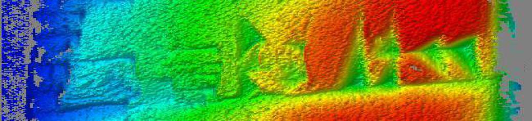
The PRM contains the information needed to generate a collection of visualization images, each highlighting a different type of 3-D shape information. The data browsing tool described above then allows the user to select landmark points, space curves, and regions of interest. The analysis is saved in what we call a Selection File, which describes, in addition to the geometric information:
- Location of the archival EOD, the "gold standard" raw sensor data.
- The user who selected those points.
- A timestamp for when they made the selection.
This allows serious data sharing and re-analysis. If I were to draw some conclusions about a specimen, I should provide you with my Selection File. That would allow you to retrieve the original sensor data as an EOD file, convert it to a PRM, and analyze just which points I selected as my landmarks. You might have selected those landmarks slightly differently, or you might have also selected other landmarks of specific interest to you. The Selection File, precisely describing my analysis in terms of the original sensor data, allows us to discuss issues quantitatively.
Here is an example of the beginning of an EOD file,
including the self-explanatory header
(those lines beginning with a "#" character)
and the first few lines of the data itself.
The complete file contains 146,209 lines, although it
compresses to 476 kbytes with the gzip utility.
## EOD-A1
## nslice = 350
## nrow   = 480
## calibration matrix =
##                          0                        0                        0
##    -0.00253057036915258805  0.000788688629679867555      2.10090292240347187
##    0.000249555848398209208    0.0059707379534091852    -0.539184509939298451
## 8.9900797933981379527559e-8 1.034813752990301086614e-5 3.9370078740157480315e-2
## start vec = 0 0 0
## shift vec = 0.12337142966 0 0
## ztwist = 0
################################################################
## History:
##  Created by table-scanner at Tue Dec 15 13:49:50 1998
##  User@System: cromwell@rvl4.ecn.purdue.edu
##  Contents: Cuneiform tablet, Spalding 1, Ur III, obverse side, roughly in middle
##  Sensor: RVL, top-down, 75mm, f/4 (noted fine-scale irregularity during scan)
################################################################
## Run-length coding is used with ASCII storage.  Explanation.
##
## The first ASCII number is the number of valid values to follow.  It
## is followed by that number of data points.
##
## The next number is the number of invalid values to follow -- it should
## be replaced by that number of zeros.
##
## This pattern of 'valid-length, data points, invalid-length' continues
## until the nslice x nrow data array is filled.
##
## The sequence:
##	0			(no initial valid points)
##	2			(two invalid points)
##	3			(three valid points)
##	1 2 3			(valid data)
##	2			(two invalid points)
##	4			(four valid points)
##	5 6 7 8			(valid data)
## Should be expanded to:
##	0 0 1 2 3 0 0 5 6 7 8
##
## The first point in the array is the top of the left-most column.
## The second point is the second-to-top point of the left-most
## column.  The columns are filled top-to-bottom, and are filled
## in left-to-right.
################################################################
## Each data point contains two values.  The first is the offset
## value, the second is (255-intensity).  It is more efficient to
## store the intensity data as (255-intensity) as value points
## from most sensors are closer to 255 than to 0, so that ASCII
## storage will be slightly lower.
##
## This means that the above sequence can now more completely
## considered as:
## The sequence:
##	0			(no initial valid points)
##	2			(two invalid points)
##	3			(three valid points)
##	1 10 2 12 3 8		(valid data)
##	2			(two invalid points)
##	4			(four valid points)
##	5 4 6 20 7 24 8 30	(valid data)
## Should be expanded to an offset data vector:
##	0 0 1 2 3 0 0 5 6 7 8
## and an intensity data vector:
##	0 0 245 243 247 0 0 251 235 231 225
##
## The first point in the array is the top of the left-most column.
## The second point is the second-to-top point of the left-most
## column.  The columns are filled top-to-bottom, and are filled
## in left-to-right.
################################################################
## RVL-style "offset data" range map storage.  Explanation:
##
## For the n'th value in the expanded list, let:
##	Stripe = int(n/nrow)
##	Row = n - Stripe*nrow
##	M = the calibration matrix defined above
##
## [x']     [ Stripe ]			 [x] = [x'/t]
## [y'] = M [ Row ]		and then [y] = [y'/t]
## [z']     [ 1.0 ]			 [z] = [z'/t]
## [t ]
##
## (For details see C.H. Chen & A.C. Kak, 'Modeling and calibration
##  of a Structured Light Scanner for 3-D Robot Vision,' Proceedings
##  of the IEEE International Conference on Robotics and Automation,
##  pp. 807-815, Raleigh NC, March 1987.
##
## For the transformation specific to slice number N, let:
##	X  = [x y z] initially calculated as above
##	X1 = the start vector
##	dX = the shift vector
##	tz = the twist angle, in degrees
##
##                    [  cos(tz*N)  sin(tz*N)  0 ]
## X = (X + X1 + dX*N)[ -sin(tz*N)  cos(tz*N)  0 ]
##                    [      0          0      1 ]
##
################################################################
## END
1
0 255
1
1
95.27 244
2
2
96.11 242
95.76 244
2
2
94.74 218
95.5 239
15
1
95.25 234
1
2
95.46 240
94.25 238

[... many more lines deleted ...]