Localized Contrast Enhancement for 3-D Visualization
3-D Data Visualization
Background
This is an application of my localized histogram equalization technique. See the page describing that technique first, to understand the image enhancement done here.
Visualizing Range Maps
A range map is a 2-D array of 3-D vectors. I have used a variety of methods for visualizing range maps. Each vector describes a location in space of a point measured with a single-plane structured-light range sensor. The 2-D array is arranged as gathered by the sensor, with each column coming from one digitized video image (thus 2-D slice). The 3-D vector stored at row r of column c is from video scan line r of frame (slice) c.
Range maps are visualized by calculating an average surface normal for the scene, and assuming that the viewpoint lies near the projection of that vector from the centroid of the measured points. In simple terms, you are looking into the measured surface(s).
The proximity to the theoretical viewpoint is defined as the dot product of the average surface normal unit vector with the vector from the scene centroid to the point in question.
If the nearest point (that for which the dot product is maximum) and furthest point (that for which it is minimum) are found, all points can be colored or darkened depending on where they lie in that continuum. I have encoded depth as intensity by using brighter colors for points near the viewpoint. For depth as hue, blue is farthest and red is nearest.
Given the local surface normal vectors, calculated from the individual surface points, and given a theorized lighting model, a rendering of the surfaces can also be generated.
Enhancing Visualization Images
Now, the distribution of ranges, which will be represented as hue or intensity, can be remapped to maximize detail. Histogram equalization is a good initial step. However, sometimes fine-scale 3-D shape is of more interest than gross shape. For two examples, finding small biological features like the relatively small spines on a fish skull. Or, highlighting the signs (plus wear and damage) on a cuneiform tablet.
Greyscale images use values in the range 0-255. True color images use only 256 values per color plane. So, a remapping that selects one of 256 values seems acceptable if our only goal is an image. Localized histogram equalization uses only the 16x16 subimage surrounding a point in question to select a remapping. For points within 8 rows or columns of an edge, the 16x16 subimage is kept entirely within the image, and thus those points are not at the center of the region which determines their remapping. The unusual step here is that the histogram equalization is applied to the range value (the dot product described above) instead of the image. The processed range is then used to generate an image in the usual way. This "equalized" range map has lost its large-scale variation in the direction of the average surface normal. It roughly resembles the effect of lifting a mask of fine-scale detail off a smooth overall form, and then draping the mask on a flat surface.
Below is a series of image pairs. The first image in each pair shows the original visualization method, and highlights overall shape. The second image shows the result of localized histogram equalization applied to the image component used to encode range, and highlights fine-scale shape. The second images also highlight sensor quantization, especially in smooth areas nearly perpendicular to the average surface normal.
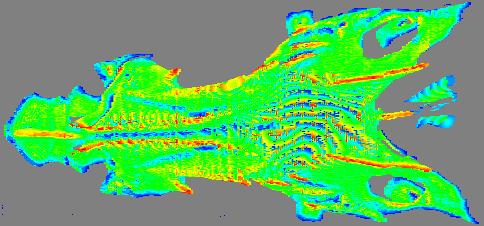
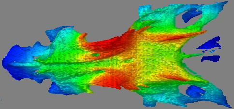
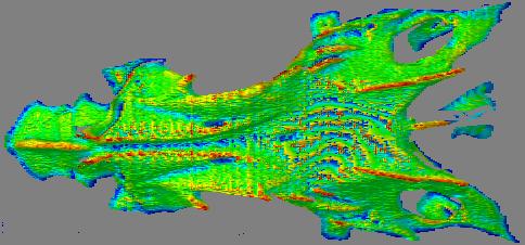
Fish Skull
Depth as intensity, large-scale.
Depth as intensity, fine-scale.
Depth as hue, large-scale.
Depth as hue, fine-scale.
Depth as hue, overlaid on the rendered local orientation, large-scale.
Depth as hue, overlaid on the rendered local orientation, fine-scale.
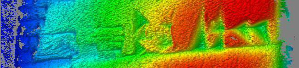
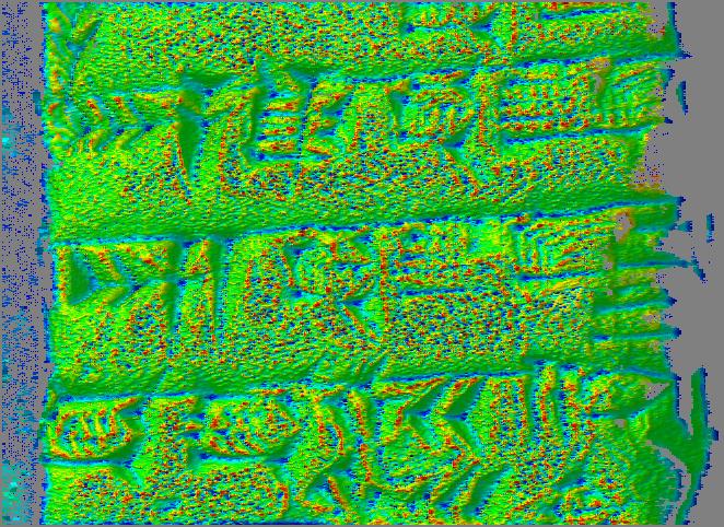
Cuneiform Tablet
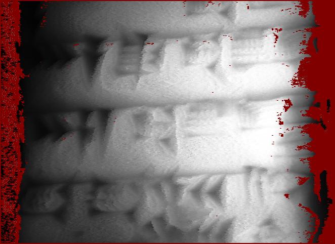
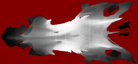
Depth as intensity, large-scale enhancement.
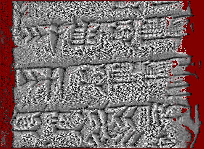
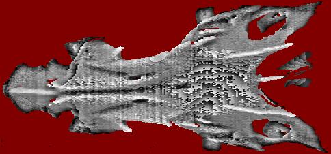
Depth as intensity, fine-scale enhancement.
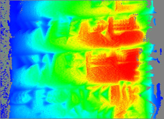
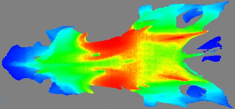
Depth as hue, large-scale enhancement.
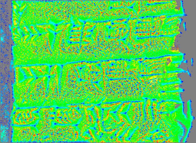
Depth as hue, fine-scale enhancement.
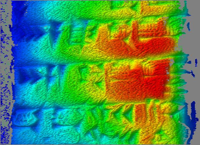
Depth as hue, overlaid on the rendered local orientation, large-scale.
Depth as hue, overlaid on the rendered local orientation, fine-scale.
Discussion
It would seem that the locally enhanced depth as intensity image is probably the most significant improvement provided by this technique. The locally enhanced depth as hue might be useful for the biological sample, but seem less useful for the cuneiform tablet. The two most useful images seem to be the depth as intensity, fine-scale, and the depth as hue overlaid on rendering, large-scale. In other words, the second and fifth in each set. The fine-scale depth as intensity makes several otherwise illegible signs visible on the cuneiform tablet. The depth as hue, both overlaid on rendering and not, makes several of the spine and ridge features visible, or at least far more prominent, on the fish skull.
Data sources and references
Data sets were:
"Dorsal view, neomerinthe hemingwayi skull, GCRL 26666"
dorsal-gcrl-26666.eod
spatial sampling: 0.083-0.30 mm
"Cuneiform tablet, Spalding 1, Ur III, obverse side,
roughly in middle"
offset.1998-12-15-13:49:50.eod
spatial sampling: 0.064-0.12 mm
The following provided the motivation and initial guidance: "Contrast Limited Adaptive Histogram Equalization," Karel Zuiderveld, Graphics Gems IV, Paul Heckbert, editor, Academic Press, 1994. However, that work described subdividing the image into 16x16 blocks, calculating the histogram of each such block, and interpolating between remappings for points. I calculated the histogram for each 16x16 block centered on a measured point, increasing the computational expense by a factor of 256. However, it still takes only about a minute on an AMD K6-333 running Linux to produce the images for the large (660 cols, 480 rows) range map of the cuneiform tablet.