Collecting 3-D Range Data and Reflectance Maps
Data Collection
There are many scientific applications for visualizing image data. Images that reveal three-dimensional shape can sometimes be used to study objects when you don't have direct physical access. This might be more subjective, to read inscriptions or interpret a sculpture's shape. Or it might be quantitative, to make accurate measurements for morphometric analysis. We just have to collect and process the data.
2-D Image Data, Then ...
Long ago, in the 1980s and early 1990s, 2-D image capture required feeding an analog video signal into a digitizer.
The NTSC analog video standard used in most of the Americas plus Japan, South Korea, Taiwan, the Philippines, Burma, and a few Pacific islands, dated back to 1941. Provisions for color were grafted onto it in 1953. NTSC provided 483 visible lines per frame, and a typical digitizer produced 512 pixels per line. The PAL and SECAM standards used elsewhere had different scan rates and bandwidth, but generally speaking when you digitized analog video you got images approximately 500×500 pixels in size. That's just 0.25 megapixels.
Bandwidth limitations in the camera and digitizer (and in the transmission cable, when the digitizer was mounted in an equipment rack a few rooms down that hall!) imposed further limits. A tightly focused point of light several meters away in a darkened room should occupy a space much smaller than a single pixel in the camera's sensor array. But the resulting region in the digitized image might be four to five pixels long along the scan lines and at least an extra pixel wider above and below the peak.
Oh, and most digitized images were monochrome. You could digitize color images, but it might involve digitizing three images taken in sequence through three color filters on a monochrome camera.
... and Today's 2-D Image Data Collection
Now everyone's camera contains a multi-megapixel color camera with excellent autofocus and low-light performance. The lenses are tiny, which actually can work to our advantage as they are closer to an idealized pinhole model.
Today's digital cameras have sensor arrays of 3200×2400 pixels and larger. That makes them significant larger than typical computer displays.
$ xdpyinfo | less
[...]

screen #0:
  dimensions:    1920x1080 pixels (508x285 millimeters)
  resolution:    96x96 dots per inch
  depths (7):    24, 1, 4, 8, 15, 16, 32
  root window id:    0x28b
  depth of root window:    24 planes
[...]
$ xdpyinfo | less
[...]

screen #0:
  dimensions:    1366x768 pixels (361x203 millimeters)
  resolution:    96x96 dots per inch
  depths (7):    24, 1, 4, 8, 15, 16, 32
  root window id:    0x80
  depth of root window:    24 planes
[...]
3-D Image Data Collection, Then...
Structured-light range sensors use a pretty simple concept. Shine a plane of light into a scene, and then observe its intersection with the scene from a viewpoint off to the side of the light plane.
It's pretty easy to see that the resulting pattern in the camera image suggests the shape of the target. But once you have calibrated the system of projector and camera, you can calculate the (x,y,z) position in the world for any (row,column) position in the camera.
This is, of course, a 2-D sensor as it can only measure points within the light plane.
Fasten the projector and camera to a fixture to make a rigid sensor assembly, so the same calibration matrix applies to every image. Now sweep that fixture past the scene, or pass the scene past the sensor on an assembly belt or similar. Digitize a series of frames and you have a 3-D sensor that has measured a cloud of points within a 3-D volume.
Assemble this data into a range map, a two-dimensional array of (x,y,z) locations, where each column comes from one digitized frame. For typical sensor geometry, the camera will see at most one intersection of the light plane per scan line, so the rows in the range map can correspond to the original scan lines.
The problem is that you have to collect a large number of frames, moving the sensor or target for each one. A useful range map will have at least a few hundred columns, or original digitized frames.
... and Today's 3-D Image Data Collection
The current way to collect 3-D range maps is to take several high-resolution pictures and use software to automatically find corresponding points. 3-D positions of the corresponding points are calculated as the camera positions are back-calculated.
Let's See Today's Data Collection Methods
2-D and 2.5-D Image Data
Polynomial Texture Mapping or PTM, also known as Reflectance Transformation Imaging or RTI, is a "2.5 dimensional" sensing technique. Several images are taken with the camera in a fixed position and orientation, with a light source moved to several positions. A standardized lighting target, a reflective metal sphere, is placed within the scene.
The result is a 2-D image which the user can illuminate in various ways, moving a virtual light source as desired. For more details see:
The Wikipedia article on polynomial texture mapping.
A paper by one of the technique's developers, hosted at HP.
The SIGGRAPH paper Polynomial Texture Maps
Examples of applications from Cultural Heritage Imaging
Archaeological applications of polynomial texture mapping: analysis, conservation and representation University of Southampton
Range Maps and 3-D Models
The goal is a cloud of points that can be raytraced as a set of facets and visualized with arbitrarity position and orientation, surface characteristics, and lighting.
Terrestrial Laser Scanning or TLS is used for applications on the scale of architecture.
Photogrammetry is one term for finding corresponding points in multiple images and calculating their 3-D positions. You will see the terms Shape from Motion and Structure from Motion (both SfM), Multi-Image Matching, and Image-based Matching (IBM) used to describe this technology.
D. Skarlatos and S. Kiparissi, Cyprus University of Technology, ISPRS Annals of the Photogrammetry, Remote Sensing and Spatial Information Sciences, Volume 1-3, 2012, XXII ISPRS Congress, 25 August – 01 September 2012, Melbourne, Australia.
I found this paper to be a good survey. They describe Multi-Image Matching as being introduced in the 1988 paper "Geometrically Constrained Multiphoto Matching" by Gruen and Baltsavias. They used Menci's Zscan, a commercial trifocal photogrammetry system, and the open-source solution based on Bundler and PMVS.
They found that the open-source Bundler–PMVS workflow was superior to the commercial Zscan system in terms of accuracy, point density, and overall model quality. Tested against an architectural façade, Bundler-PMVS outperformed a laser scanner.
Also see:
Towards High-Resolution Large-Scale Multi-View Stereo, Vu Hoang Hiep, Renaud Keriven, Patrick Labatut, and Jean-Philippe Pons, IMAGINE, Université Paris-Est, LIGM/ENPC/CSTB, ENSAM, Cluny.
A Simple Prior-Free Method for Non-Rigid Structure-From-Motion Factorization, Yuchao Dai, Hongdong Li, and Mingyi He, Northwestern Polytechnical University, Australian National University, Australia.
Example Data
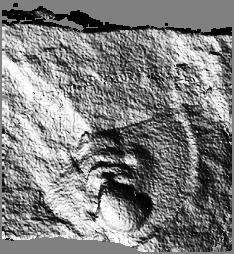
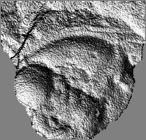
These are rendered range maps. A 2-D array of (x,y,z) points was collected with a single-plane structured light sensor. Surface normals were calculated and used to generate a simulated image.
The object is a fossilized trilobite embedded within a flat stone surface.
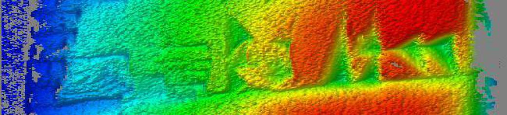
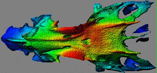
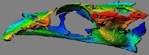
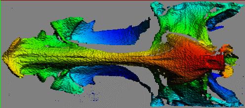
These are also rendered range maps. The local surface orientation relative to a theorized viewpoint (looking straight into the picture) and lighting vector (from our upper left) generates the intensity.
Depth along the viewing vector generates the hue, red is closest and blue furthest away.
The object is a skull of a Neomerinthe Hemingwayi, one of a genus of scorpionfishes.
These are raytraced 3-D data sets for a similar Neomerinthe hemingwayi skull. The first image here shows how data from three viewpoints was integrated.
The points from the green, blue, and purple data sets were registered and merged into the same data set. Raytracing was done on a Silicon Graphics workstation.
In the first image the facets from the three data sets are assigned unique colors.
In the second image all facets have been assigned the same more realistic color model.
These are rendered range maps of a cuneiform tablet. The same tablet, and the same underlying range map. The different is that the surface normals have been calculated over different sizes of surface patches.
Larger patches were used on the second image, causing more smoothing.
These are range maps of a US $0.01 coin, visualized in two ways.
In the first of each image pair, depth is coded as intensity — white is the closest of the data set to the camera, black is furthest.
In the second of each pair, depth is coded as hue from red to blue, while intensity models the local surface orientation with a theorized light source to our upper left.
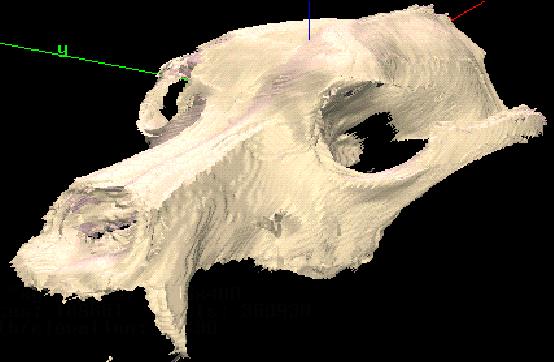
This is the result of mergining six data sets. A dog skull was placed on a turntable and scanned at six orientations 60° apart.
The six data sets — red, green, yellow, light blue, dark blue, and purple — were merged and raytraced on a Silicon Graphics workstation.
The first image shows the contributions of the six data sets, the second is the result of giving all six the same realistic reflectance model.