Calculating Surface Normals and Curvatures

Starting with the range map

Range map visualization, and many types of automated analysis, require the calculation of local surface orientation (the normal vector) and also — ideally — the accurate detection of surface discontinuities, or edges.

The range map is X — this is a two-dimensional array of three-dimensional vectors, each representing a local (x,y,z) measurement if such a measurement could be made, or identical to (0,0,0) to indicate an invalid point where no measurement could be made. We will refer to the (x,y,z) measurement at range map index row, col as X_row,col.

Traditional approaches make a number of inappropriate assumptions about range data. First, that adjacency relationships in the range map correspond to adjacency relationships in the real world. This really implies three underlying assumptions:

• Jump discontinuities do not exist.

• Small local extrema do not exist.

• Sensor sampling was dense enough to capture all surface features.

Traditional approaches also assume that the spatial sampling rates along both columns and rows are roughly equal and constant throughout the range map.

The Surface Normal

The surface normal is a unit vector perpendicular to the local surface. We can calculate a map of surface normals, a two-dimensional array of surface normal vectors, where S_row,col is the surface normal at range map index row,col. The surface normal indicates how the measured surface location varies while indexing across the range map, and so it is the first derivative of position:
     S = dX/dindex
where index is some measure of location within the map.

The Curvature

The curvature indicates how the surface orientation changes as one traverses the surface. Put another way, it indicates how the surface normal change with index across the range map. Therefore the curvature is the derivative of the surface normal, and thus the second derivative of position:
     C = dS/dindex = d²X/dindex²

Traditional Methods of Calculating Surface Normal and Curvature

Traditional methods for calculating surface normal and curvature start by convolving the range map X with various 3x3 kernels, then combining the resulting terms. 5x5, 7x7, or even larger kernels could be used to reduce noise; this is effectively the same as first smoothing X with a 3x3, 5x5, or larger smoothing kernel, and then applying the convolutions that calculate partial derivatives.

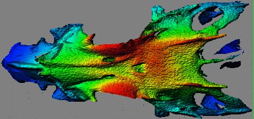
A variation on this is to observe that each range point belongs to 9 3x3 patches (or to 25 5x5 patches, or 49 7x7 patches, or...), and to calculate the normal and curvature for each of them. Then, for the point in question, use the measures from the patch that is most planar. If the target is known to be made up of roughly planar regions, this modification may help. But smoothly curving surfaces end up with a faceted appearance if this assumption is inappropriately applied. The result is a "contour map" effect, as seen below in the dorsal view of a fish skull (the skull is seen from above, with the nose of the fish to the left). Note the "contour map" effect in the nearly flat region at the top of the head behind the eye sockets, and the general graininess of the rendered surface.

The Signal Processing View, and What is Wrong With Traditional Techniques

Since normals and curvatures are first and second derivatives, respectively, we must keep in mind that a derivative is a high-pass filter. A second derivative is a high-pass filter with a faster roll-off.

If we are really discussing filters, it would be appropriate to ask about the cutoff frequency (or wavelength) and the roll-off. For instance, "a high-pass filter with 3-dB cutoff frequency of 10.8 MHz and a roll-off of 16 dB per decade", as we might specify a conventional filter.

We cannot answer these questions in any meaningful way! The spatial sampling rates along rows and columns are unequal:
     dX/drow != dX/dcol
The spatial sampling rates along either rows or columns varies throughout the image, so in some sense dX/drow is not equal to dX/drow when measured at different parts of the range map.

Furthermore, the traditional methods of calculation were devised in a time when range maps were only as large as absolutely necessary. In other words, the data sampling was as coarse as possible to achieve the goal with a minimum of data collection and processing. With increasing computation and storage capabilities, modern data frequently has dX/drow and dX/dcol close to the spatial sampling limits of sensor geometry and optics.

Applying a 3x3 convolution to finely sampled data yields very localized measures. In signal processing terms, the roll-off frequency is very high. Speaking practically, or esthetically, the result will be of little use as it will be dominated by small-scale high-frequency noise, as seen below.

The Solution for Calculating Surface Normals

First, we must calculate local index-based "derivatives", which of course are not really derivatives at all but merely differences.
     δX/δrow = X_row+1,col - X_row,col
     δX/δcol = X_row,col+1 - X_row,col

Then, calculate local estimates of dX/drow and dX/dcol based on weighted averages of δX/δrow and δX/δcol. These weighted averages are calculated over collections of points that lie within some specified distance of the point in question. The weight varies linearly with distance from that point. The specified distance, or radius of interest, is based on the scale of the features of interest.

In words, to calculate dX/drow for some specific r,c index in the range map, let us select some range of interest R, where R is approximately the size of the target features that interest us. Next, find the set of points in the range map within R of the point at index r,c. Note that this distance is in real-world coordinates, not in the indices of the range map, and it consists of finding all range map indices i,j where:
     | X_r,c - X_i,j | < R

For each point i,j we must calculate a scaling factor S:
     S = 1.0 - | X_r,c - X_i,j |/ R
In other words, the contribution of points decreases linearly with distance, reaching zero at distance R

We then sum the scaled contributions of δX/δrow and δX/δcol, dividing each by the sum of the scaling factor S, to estimate dX/drow and dX/dcol on a physically meaningful scale. Note that these derivatives are vectors:

for (each row, col index) {
    dXrow,col/drow = 0
    dXrow,col/dcol = 0
    sum = 0
    for (each i, j index where | Xr,c - Xi,j | < R) {
        S = 1.0 - | Xr,c - Xi,j |/R
	dXrow,col/drow = dXrow,col/drow + S*δXi,j/δrow
	dXrow,col/dcol = dXrow,col/dcol + S*δXi,j/δcol
        sum = sum + S
    }
    dXrow,col/drow = (dXrow,col/drow)/sum
    dXrow,col/dcol = (dXrow,col/dcol)/sum
}

Given these derivatives dX/drow and dX/dcol, we can calculate the local surface normal N as their cross product:
     N_i,j = dX_i,j/drow x dX_i,j/dcol,

The Solution for Calculating Curvatures

The curvature C can be estimated as follows, where "·" specifies the dot product operator:
     d²X_r,c/drow² = ( X_r+1,c - X_r,c) · N_i,j - ( X_r,c - X_r-1,c) · N_i,j
     d²X_r,c/dcol² = ( X_r,c+1 - X_r,c) · N_i,j - ( X_r,c - X_r,c-1) · N_i,j
This is noisy, so again it should be smoothed over linearly scaled regions based on actual range from the point of interest, as was done to calculate normals.

Example Results

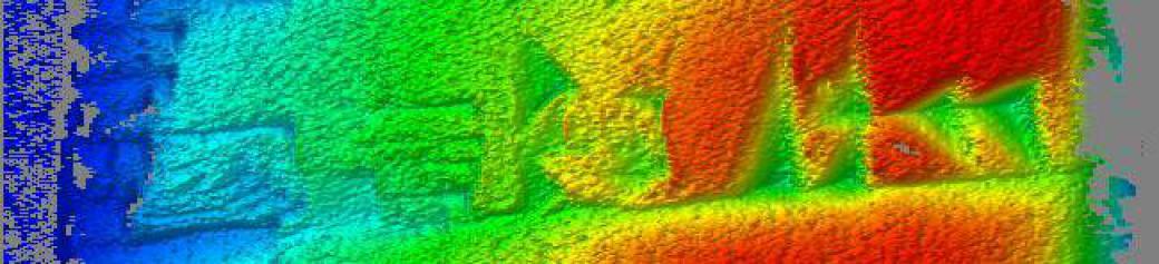
The example target is a cuneiform tablet.

Overall tablet dimensions are approx 30x30 mm.

Lines of cuneiform text are spaced approximately 7-10 mm apart.

Individual signs are approximately 5-7 mm on a side. Wedges are approximately 1.2 x 5 mm. Circular pits are approximately 3.5 mm in diameter.

The following are rendered images based on normals calculated in different ways. First, using the traditional method, showing the graininess. Then at a variety of scales corresponding to the scales of sign components, signs, and the overall tablet.

Original method — note graininess

R = 0.20 mm, approximate scale of sign components

R = 1.00 mm, approximate scale of signs

R = 3.00 mm, individual signs are lost and overall shape is shown

Further Details Regarding Curvature

The traditional method calculated d²X/drow² and d²X/dcol², and then combined them. This assumed that interesting features were aligned with either the range map rows or columns. But how should we really do this?

Our method is to calculate four terms — along rows, along columns, and along both diagonals:

• d²X/drow²
• d²X/drowdcol
• d²X/dcoldrow
• d²X/dcol²

Some features will only appear in one of these four measures.

As a single curvature measurement, we could select at each row,col index the one measure with the greatest magnitude. Or, we could simply use the average of the four. While the results are very slightly different, there seems to be no significant difference in data quality. Below are the results for curvature measurements at scales of 0.3 mm, 0.5 mm, 1.0 mm, and 3.0 mm.

R = 0.30 mm

R = 0.50 mm, approximate scale of sign components

R = 1.00 mm, approximate scale of signs

R = 7.00 mm, individual signs are lost and overall shape is shown

Further Results

Below are some images that suggest that the curvature measurements described here can highlight some detail that would unseen in a rendered image. A rendered image must specify some lighting vector, and one combination of lighting and view vectors will always leave some 3-D features unseen.

The curvature image (at left) clearly shows that there are four semicircular sign components, while the rendered image (at right) is a bit confusing.

The curvature image (at left) clearly shows that the left-most column has three wedges, while the middle wedge is difficult to see in the rendered image (at right).

While the curvature image (at left) looks a bit "noisy", it does reveal some sign components that are difficult to see in the rendered image (at right).

Conclusions

The methods described here are more computationally expensive. However, this is of little concern with modern computer speeds, and it will only become less of a concern over time.

It appears that this method would be worth the computational expense for certain applications:

• Accurate visualization of densely sampled range maps
• Cueing a human user to find areas of interest
• Automatically selecting points of interest to be used for automated registration (e.g., ICP)

Other Related Work

Adaptive local extrema detection.